GPU text rendering with vector textures

Sat, Jan 2, 2016

This post presents a new method for high quality text rendering using the GPU. Unlike existing methods it provides antialiased pixel accurate results at all scales with no runtime CPU cost.

Click here to see the WebGL demo

Font atlases

The standard way of rendering text with the GPU is to use a font atlas. Each glyph is rendered on the CPU and packed into a texture. Here’s an example from freetype-gl:

Packed font atlas. Source: freetype-gl.

The drawback with atlases is that you can’t store every glyph at every possible size or you’ll run out of memory. As you zoom in the glyphs will start to get blurry due to interpolation.

Signed distance fields

One solution to this is to store the glyphs as a signed distance field. This became popular after a 2007 paper by Chris Green of Valve Software. Using this technique you can get fonts with crisp edges no matter how far you zoom in. The drawback is that sharp corners become rounded. To prevent this you’ll need to keep storing higher resolution signed distance fields for each glyph, the same problem we had before.

Artifacts from low resolution signed distance field. Source: Wolfire Games Blog.

Vector textures

The previous two techniques were based on taking the original glyph description, which is a list of bezier curves, and using the CPU to produce an image of it that can be consumed by the GPU. What if we let the GPU render from the original vector data?

32 bezier curves forming the letter H.

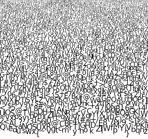
GPUs like to calculate lots of pixels in parallel and we want to reduce the amount of work required for each pixel. We can chop up each glyph into a grid and in each cell store just the bezier curves that intersect it. If we do that for all the glyphs used in a sample pdf we get an atlas that looks like this:

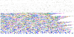
Vector atlas for 377 glyphs.

Despite looking like a download error, this image is an atlas where the top part has a bunch of tiny grids, one for each glyph. To avoid repetition, each grid cell stores just the indices of the bezier curves that intersect it. Bezier curves are described by three control points each: a start point, an end point and an off-curve point¹. The bottom half of the image stores the control points for all beziers in all glyphs². All we need to do now is write a shader that reads the bezier curve control points from the atlas and determines what color the pixel should be.

A bezier curve shader

Our shader will run for every pixel we need to output. Its goal is to figure out what fraction of the pixel is covered by the glyph and assign this to the pixel alpha value³. If the glyph only partially covers the pixel we will output an alpha value somewhere between 0 and 1 — this is what gives us smooth antialiasing.

We can treat each pixel as a circular window over some part of the glyph. We want to calculate the area of the part of the circle that is covered by the glyph.

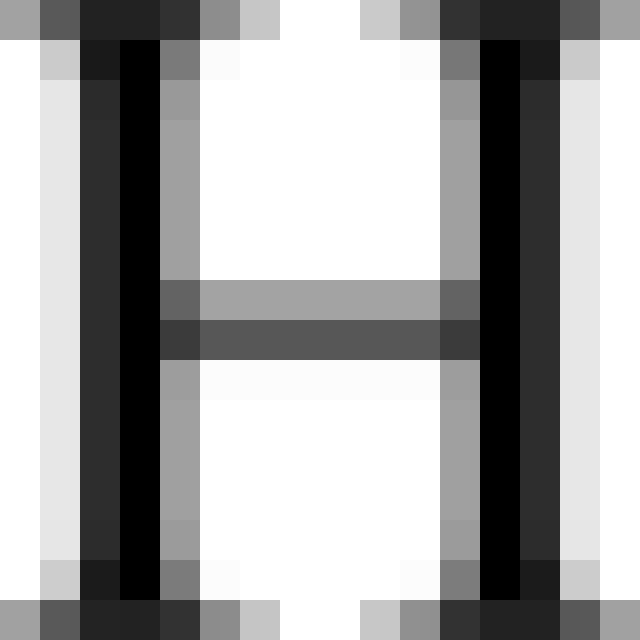
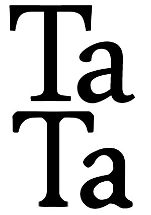
The desired result at 16 by 16 pixels.

Treating the pixel window as a circle⁴, our task is to compute the area of the shape formed by the circle boundary and any bezier curves passing through it. It’s possible to compute this exactly using Green’s theorem, but we’d need to clip our curves to the window and make sure we have a closed loop. It all gets a bit tricky to implement in a shader, especially if we want to use an arbitrary window function for better quality⁵. However if we reduce the problem to one dimension it becomes a lot more tractable.

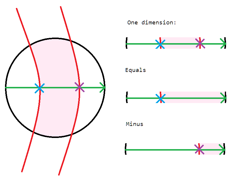
Two curves passing through a pixel window. The area of the shaded region can be approximated by looking at its intersections with a ray passing from left to right. Source: MS Paint.

The idea is to take a ray passing from left to right. We can find all the intersections of this ray with all the bezier curves⁶. Each time the ray enters the glyph we add the distance between the intersection and the right side of the window. Each time the ray exits the glyph we subtract the distance to the right side of the window⁷. This gives us the total length of the line that is inside the glyph, and will work for any number of intersections or bezier curves.

More samples for more accuracy

The result may be inaccurate if our horizontal ray intersects the bezier curves at a glancing angle. We can compensate for this by sampling several angles and averaging the results⁸. This gives a robust approximation of the 2D integral⁹.

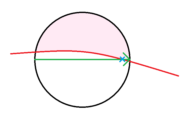
Underestimation of covered area due to a curve intersecting the horizontal ray at a glancing angle. The shaded area is close to half the pixel but the estimate from this horizontal ray is much lower.

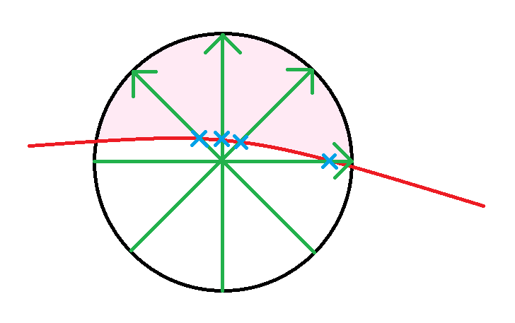
Increasing accuracy by sampling at several angles.

In practice only a few samples gives a high quality result. To see why supersampling helps we can make the pixel window very large:

Why supersampling is needed. Clockwise from top left: 2, 4, 8, 16 samples. The integration window here is larger than it should be to make the errors more visible. The error is less noticeable when the window is only one pixel — the demo uses four samples.

Demo

If you have a device that supports WebGL you can see a proof of concept demo here.

This technique is harder on the GPU than atlas textures but avoids the need to use the CPU to render at runtime when a required glyph size is missing. It can also deliver higher image quality: atlas textures have the drawback that when text is scaled, rotated or shifted by a subpixel amount there is no longer a 1:1 correspondence between screen pixels and atlas texels.

See here for some implementation notes on the demo.

Quadratic beziers have 3 control points, cubic beziers have 4. Fonts may use either depending on format, but we can preconvert cubic curves to multiple quadratic curves with arbitrary accuracy. The shader could be modified to deal with cubic beziers directly — this would require finding roots of cubic polynomials instead of quadratics. ^[return]
The bezier data is one dimensional and would be better stored in a buffer texture or SSBO but WebGL does not yet support these. ^[return]
This is equivalent to convolving the glyph with a one pixel rectangular window (box filtering). We can actually use any window function; the demo uses a parabolic window. ^[return]
Despite often being represented as squares when an image is blown up, pixels are point samples and shouldn’t be treated as a square region. See A Pixel Is Not A Little Square by Alvy Ray Smith. ^[return]
See this 2013 paper by Manson and Schaefer for a method that uses boundary integrals to rasterize curves on the CPU. ^[return]
The intersections of a quadratic bezier and a horizontal line can be found cheaply using the quadratic formula. ^[return]
We can tell which side of a bezier curve is inside the glyph by sticking to a convention for the control point order. For example: travelling from the start point to the end point, the inside of the glyph is always to the right. ^[return]
Instead of rotating our ray, we can rotate the bezier curves. Rotating a bezier curve is quite easy to do: we simply rotate its control points. In fact with this technique our window doesn’t have to be circular. We can apply any affine transformation to the control points, letting us integrate over any oriented ellipse. The screenspace derivatives of our sample coordinates give the required transformation. This allows us to correctly antialias stretched, skewed, rotated or perspectively projected glyphs. See here for a example of how this works. The green and red lines are the screen space derivatives. ^[return]
Another way to think about this is that each sample represents a (double) wedge-shaped portion of the circle, and we are summing them to get the full circle. The more samples we take the smaller the wedges are and the more accurate our approximation is. The demo actually analytically integrates these wedges multiplied by a spatial filter, starting at the intersection point. ^[return]

Will Dobbie